Asphaltene Deposition

Once asphaltene deposition is identified in the field or there is a reason to believe that this problem is imminent as a result of gas injection, for example, active mitigation strategies are needed, which are usually based on continuous injection of various types of asphaltene deposition inhibitors (usually called “asphaltene inhibitors”). The most common types of asphaltene inhibitors are dispersants. Thus in this work we use “asphaltene inhibitor” as a general term to refer to chemicals that intend to mitigate asphaltene deposition and “asphaltene dispersant” a particular type of asphaltene inhibitor, whose mechanism of action is the dispersion of asphaltene aggregates. The utilization of asphaltene dispersants has shown mixed results in the field and in several cases it has been reported that the addition of dispersants can worsen the asphaltene deposition problem. For example, Juyal et al. (2010) reported an increase in the amount of asphaltene deposit collected in a Taylor-Couette cell operated at high shear, and at high pressure and temperature, after addition of two chemicals that were expected to mitigate asphaltene deposition. At concentrations of 500 ppm, Chemicals A and B showed an increase of 17 and 100% on the amount of deposit collected at the end of the experiment, respectively.

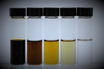
The current testing procedure that is widely used to assess the performance of chemicals is to blame for the poor performance of these chemicals under more realistic conditions. This method, known as the Asphaltene Dispersion Test (ADT), is depicted in Figure 1. ADT uses dead oil samples at ambient conditions to evaluate the ability of a given chemical to delay asphaltene sedimentation upon addition of n-heptane in a 24-hour period. Although this technique is used to screen various chemicals at different dosages, there are several shortcomings that make this method unsuitable for practical application: a. The analysis is done at ambient temperature, b. The oil sample is highly diluted, c. Delayed sedimentation is not an indication of reduced deposition. Actually, it is now well-accepted that the smaller the asphaltene particles the more their tendency to deposit (Vargas, 2010; Akbarzadeh, 2011).

Figure 1. Asphaltene Dispersion Test (Melendez, 2015).

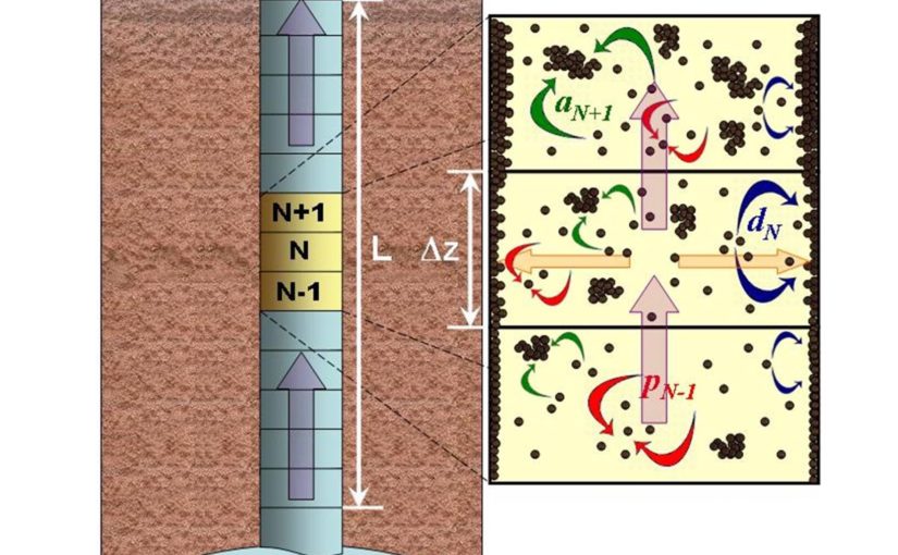
Lin et al. (2015), from the Biswal group at Rice, showed that the addition of the best dispersant selected from a group of 15 chemicals using the ADT produced, increased asphaltene deposition, according to Figure 2. Melendez et al. (2015), from the Vargas lab group at Rice University, designed and fabricated a novel setup to probe asphaltene deposition under dynamic conditions, whose schematic is shown in Figure 3. This preliminary setup, which was built as a proof of concept, has been used at ambient temperature and pressure. This system is composed by a multi-section column that can be packed with spheres of any given material, e.g. carbon steel. By changing the number and the size of the spheres and the number of sections, the surface area for asphaltene deposition can be efficiently adjusted. PTFE was the selected material for the tubing, the column shell, fittings and valves, to minimize asphaltene interactions and for the good resistance to organic solvents. Variables that can be manipulated in this system are: flow rates, ratio of oil to precipitant, concentration and type of inhibitor, surface area for asphaltene deposition, and the number of pore-volumes. Another significant advantage of the new setup over alternative methods is the possibility of investigating the effect of water, pH and electrolyte content on the precipitation and deposition of asphaltenes, and any potential interactions between water and asphaltene dispersants, or asphaltene and asphaltene dispersants in the presence of water. Moreover, other important applications of the new system may include the analysis of the effectiveness of surface coatings to reduce asphaltene deposition or to analyze the interrelation between corrosion and asphaltene deposition, among others. A new setup to perform experiments at high pressures and temperatures can be built, using materials that can withstand corrosion such as titanium or hastelloy, depending on the particular needs of the project.



Figure 2. Increased asphaltene deposition caused by the addition of a dispersant.



Figure 3. Schematic for novel multi-section packed column to probe asphaltene deposition.

The setup shown in Figure 3 has been already used to evaluate the performance of three commercial dispersants, namely 8, 9 and 15 to reduce asphaltene deposition. For this effect a dead oil sample from the Middle East (oil S) was mixed with n-heptane at a ratio of 30 parts of oil and 70 parts of n-heptane. The ratio of precipitant to oil is set above the onset of asphaltene precipitation, which can be accurately determined using the indirect method. Different experiments were conducted to quantify the amount of asphaltene deposit collected when the various dispersants are used. For all the experiments a constant flow rate of 12 ml/h of the mixture of oil and n-heptane was used and the duration of the experiment was 6 hours.

The performance of the three chemicals 8, 9 and 15 to disperse asphaltenes was also assessed by measuring the light transmittance of the samples at a wavelength of 1100 nm, and at different ratios of heptane / oil. Because the effect of dilution upon addition of heptane has been removed from the measured values, the normalized light intensity is equal to one when no asphaltene precipitation occurs, which, according to Figure 4, for this sample, corresponds to concentrations of n-heptane of 40 vol% or less. At higher concentrations of n-heptane asphaltenes precipitate out, which causes a decrease of the light transmittance. A perfect dispersant would keep the normalized light intensity at one for any concentration of n-heptane. The poorest dispersant would give the same profile as the blank. Thus, from the three tested chemicals, chemical 8 is the best dispersant and chemical 15 is the worst dispersant.



Figure 4. Normalized light intensity at 1100 nm for blends of crude oil S and n-heptane in the presence of different dispersants at ambient pressure and temperature.

A dispersion performance efficiency (DPE) for a given dispersant can be calculated according to Eq. (1). The areas ADisp and ABlank in Eq. 1 and Figure 5 are related to the change on the transmittance of light due to the precipitation of asphaltene with and without the presence of the dispersant, respectively. For a perfect dispersant ADisp should be equal to zero and DPE = 100 %, whereas in the case of the poorest dispersant, where ADisp = ABlank, DPE = 0 %.



Figure 5. Experimental determination of the dispersant performance efficiency (DPE). (a) The red area is related to the performance of a given dispersant, (b) the blue area is for the blank (no-dispersant). The smaller the red area, the better the dispersion efficiency of the given dispersant.

Figure 6 shows the amount of asphaltene deposit collected in the setup depicted in Figure 3 for crude oil S, for the case with no dispersant and for the three dispersants 8, 9 and 15. The mass of asphaltene collected in each case is plotted against the corresponding DPE.



Figure 6. Asphaltene Deposition collected from crude oil S, as a function of the DPE. Ambient T & P.

The results presented in Figure 6 are in agreement with the results from the microfluidic experiment, qualitatively shown in Figure 3. Dispersant 8, which was the best dispersant from the series of 15 chemicals tested using the ADT, increased the amount of asphaltene deposit. On the other hand, dispersant 15, which had a very low DPE value of less than 10%, is able to reduce the amount of asphaltene deposition in almost 50%. Therefore, according to these experiments, the ability of a chemical to disperse asphaltenes is not an indication of their efficiency to reduce asphaltene deposition. In many cases this relationship is actually reversed. For this reason it is of utmost importance to assess the performance of asphaltene inhibitors on their ability to reduce actual deposition (not their dispersion efficiency), under dynamic conditions and at temperatures that are relevant to the production conditions.

References

• Akbarzadeh, K., Eskin, D., Ratulowski, J., et al. (2011). Asphaltene Deposition Measurement and Modeling for Flow Assurance of Subsea Tubings and Pipelines. Presented at the OTC Brasil, Offshore Technology Conference. http://doi.org/10.4043/22316-MS



• Eskin, D., Ratulowski, J., Akbarzadeh, K., et al. (2011). Modelling asphaltene deposition in turbulent pipeline flows. Can. J. Chem. Eng., 89 (3), 421–441.



• Juyal, P.; Yen, A.T.; Rodgers, R.P.; Allenson, S.; Wang, J. and Creek, J. Compositional Variations between Precipitated and Organic Solid Deposition Control (OSDC) Asphaltenes and the Effect of Inhibitors on Deposition by Electrospray Ionization Fourier Transform Ion Cyclotron Resonance (FT-ICR) Mass Spectrometry Energy Fuels 2010, 24, 2320–2326



• Khaleel, A., Rashed, M. A., Mathew, N. T., et al. (2013). Novel Approach to Study the Instability of Asphaltenes in Crude Oil. Presented at the ADNOC Res. Dev. Acad. Conf. ARDAC, Abu Dhabi, United Arab Emirates.



• Lawal, K. A., Crawshaw, J. P., Boek, E. S., et al. (2012). Experimental Investigation of Asphaltene Deposition in Capillary Flow. Energy & Fuels, 26 (4), 2145–2153.



• Lin, Y J. , Tavakkoli, M., He, P., Ji, S Y., Mathew, N., Fatt, Y Y., Chai, J., Goharzadeh, A., Vargas, F. M. and Biswal, S. (2015), Probing Asphaltene Deposition Using Microfluidic Devices, 2015 AIChE Spring Meeting, Austin, TX, April 26-30, 2015



• Lin, Y.J., He, P., Tavakkoli, M., Mathew, N.T., Fatt, Y.Y., Chai, J.C., Goharzadeh, Vargas, F.M., and Biswal, S.L. (2016), Examining Asphaltene Solubility on Deposition in Model Porous Media”. Langmuir, 32 (34), 8729-8734.



• Melendez, Ariana M. “Experimental study of the effect of commercial dispersants on the precipitation, aggregation and deposition of asphaltenes”. M.S. Thesis, Rice University, 2015.



• Rogel, E. (2010). Effect of Inhibitors on Asphaltene Aggregation: A Theoretical Framework†. Energy & Fuels, 25 (2), 472–481.



• Tavakkoli, M., Boggara, M., Garcia M., et al. “Advances in understanding, predicting and mitigating asphaltene deposition during oil production” in “Exploration and Production of Petroleum and Natural Gas.” Editor: M.R. Riazi, ASTM. ISBN: 978-0-8031-7068-1



• Zougari, M., Jacobs, S., Ratulowski, J., et al. (2006). Novel Organic Solids Deposition and Control Device for Live-Oils: Design and Applications. Energy & Fuels, 20 (4), 1656–1663.

 

Novel Method to Detect the Precipitation of Asphaltenes

Tavakkoli and Vargas (2015) developed a new method to determine the onset of asphaltene precipitation, which is much more sensitive than current commercial techniques. In this method, which was published by Tavakkoli et al. (2015), asphaltene precipitation is detected indirectly. After the different blends of crude oil and precipitant are prepared, and certain time has elapsed to allow asphaltenes aggregates to form, the samples are centrifuged at about 10,000 relative centrifuge force for 15 minutes, which is enough to settle particles as small as 100 nm. The separation of these particles, in turn, affects the absorbance of the supernatant fluid, which can be determined in the visible region of the light spectrum, at 700 nm, or in the NIR region, at 1,100 nm. After removing the effect of dilution caused by the addition of n-heptane (and toluene that is added to stabilize asphaltenes and decrease the darkness of the sample), the absorbance of the different samples can be plotted as a function of the volume % of n-heptane. Figure 1 shows the results of this method applied to a model oil system (0.5 wt% of asphaltenes extracted from crude oil from Middle East in toluene).

According to this method, this particular oil requires the addition of 42 volume % of n-heptane to start the precipitation of asphaltenes at ambient temperature. Figure 1 also shows the excellent reproducibility of this technique. The average standard deviation (ASD) for this set of experiments is about 2 %.

The indirect method for asphaltene precipitation detection is much more sensitive than the conventional techniques based on direct determination of the presence of asphaltene aggregates (e.g. NIR light scattering), as it is shown in Figure 2. For the same model oil system, the indirect method reports an onset of precipitation of 38 volume %, whereas the direct observation of aggregates reports 44%.

Figure 1. Determination of the onset of asphaltene precipitation in a model oil system (0.5 wt% Middle East asphaltenes in toluene), using the indirect method at ambient temperature.

Figure 2. Onsets of asphaltene precipitation determined by the new indirect method and the conventional direct method for a model oil (0.5 wt% Middle East asphaltenes in toluene), at ambient temperature.

The indirect method has been successfully applied to real crude oil systems, with asphaltene contents ranging from 0.2 wt % to 10 wt %. Other advantages of this method include its ability to incorporate the analysis of the effect of water and electrolytes on asphaltene stability and to give an indication of the amount of asphaltene precipitated, not only the onset of precipitation.

References

• Tavakkoli, M., Grimes, M. R., Liu, X., et al. (2015). Indirect Method: A Novel Technique for Experimental Determination of Asphaltene Precipitation. Energy & Fuels, 29 (5), 2890–2900.

 

Asphaltene Deposition

Asphaltene precipitation is a necessary but not a sufficient condition for deposition. Additional work has been conducted to develop experimental and modeling tools to understand and predict asphaltene deposition in the production tubing (Vargas, 2010; Kurup, 2011; Akbarzadeh, 2011; Eskin, 2011).

Figure 1 shows a schematic of the multi-step mechanism for asphaltene precipitation, aggregation and deposition that is believed to occur in the wellbore. According to Vargas (2010) when asphaltenes first precipitate, they can form small aggregates called primary particles, which, in turn, can further aggregate or travel to the inner surface of the production tubing and deposit. The rate of asphaltene precipitation depends on the solubility of asphaltenes at a given pressure, temperature and composition, which can be calculated using the PC-SAFT equation of state. Additional parameters are required to establish the magnitude of asphaltene precipitation, aggregation and deposition rates, which are usually tuned to available data, either from the laboratory or the field.



Figure 1. Schematic for the multi-step mechanism for asphaltene precipitation, aggregation and deposition in a production well (Vargas, 2010).

Kurup et al. (2011) further developed the concepts proposed by Vargas (2010) to establish a one dimensional simulation tool called Asphaltene Deposition Tool (ADEPT), which was successfully used to forecast the occurrence and calculate the magnitude and profile of asphaltene deposition in the some case studies. ADEPT can be an excellent simulator to enable operators to perform quick sensitivity studies and map out operating conditions to better identify potential asphaltene deposition risks.

References

• Akbarzadeh, K., Eskin, D., Ratulowski, J., et al. (2011). Asphaltene Deposition Measurement and Modeling for Flow Assurance of Subsea Tubings and Pipelines. Presented at the OTC Brasil, Offshore Technology Conference. http://doi.org/10.4043/22316-MS



• Eskin, D., Ratulowski, J., Akbarzadeh, K., et al. (2011). Modelling asphaltene deposition in turbulent pipeline flows. Can. J. Chem. Eng., 89 (3), 421–441.



• Khaleel, A., Rashed, M. A., Mathew, N. T., et al. (2013). Novel Approach to Study the Instability of Asphaltenes in Crude Oil. Presented at the ADNOC Res. Dev. Acad. Conf. ARDAC, Abu Dhabi, United Arab Emirates.



• Kurup, A. S., Vargas, F. M., Wang, J., et al. (2011). Development and application of an asphaltene deposition tool (ADEPT) for well bores. Energy Fuels, 25 (10), 4506–4516.



• Vargas, F.M., Creek, J.L., & Chapman, W.G. (2010), On the Development of an Asphaltene Deposition Simulator, Energy & Fuels, 24 (4), pp 2294-2299. http://doi.org/10.1021/ef900951n

 

Asphaltene Precipitation Modeling: Detection of Experimental Inconsistencies

Asphaltene precipitation and subsequent deposition is a flow assurance problem that, unlike wax and gas hydrate formation, is not fully understood and available mitigation strategies are not well established and in many cases are performed on a trial and error basis. Also, unlike other flow assurance issues, simulation tools for asphaltene deposition are not commercially available and current commercial packagesthat are used to predict the precipitation of asphaltenes lack the predictive capabilities that are required to distinguish between problematic and non-problematic wells.

In the last ten years, a modeling technique to predict the occurrence and the magnitude of asphaltene precipitation at high pressure and temperature based on the Perturbed Chain version of the Statistical Associating Fluid Theory (PC-SAFT) has been well established and extensively tested. This modeling technique can simulatestandard PVT experiments as well as the asphaltene onset pressure (AOP) for live oils and its blends with hydrocarbon gas (lean and rich gases) and carbon dioxide. Furthermore, the effect of oil based mud contamination, commingling of oils, and even the compositional grading produced in reservoirs that can lead to the formation of tar-mats can be quantitatively predicted with this modeling approach.

Figure 1 shows the prediction of bubble pressure and asphaltene precipitation curves for a light fluid upon injection of various amounts of lean gas.



Figure 1.Prediction of AOP for light crude oil at different temperatures and gas injections.

The modeling method using the PC-SAFT EOS was successful in correlating data at different conditions and predicting potential experimental discrepancies. In this case study, the oil operator was able to successfully reduce the number of experiments required for a complete understanding of the effect of temperature and composition on the AOP and identify and correct experimental shortcomings that otherwise could have been easily missed. For instance, in this case, the simulation parameters were tuned to data obtained for the live oil sample with no gas added, and predictions for 5%, 10% and 20% gas injection were made. The simulation results for the 10% injection case show a significant deviation from experimental values of AOP and BUBP at 255°F, while the simulation results for the 20% case show an excellent agreement. Therefore, the experimental results for the 10% case are deemed inconsistent. After the service laboratory repeated the experiments for 10% gas injection, it was possible to confirm that the first experiment was indeed flawed. Thus, once again, the PC-SAFT EOS, in conjunction with a minimum set of reliable experimental data, can be a powerful tool to design and validate expensive and time-consuming high temperature AOP experiments.

Once the right set of simulation parameters is established, not only AOP and BP curves can be determined but also all kind of PVT properties from conventional experiments such as constant composition expansion, differential liberation, separator test and swell-test.

Contact us for more information about the capabilities of our simulation tools to perform predictions of PVT and asphaltene precipitation at high pressures and temperatures.

References

• M. Abutaqiya, S. Panuganti, F.M. Vargas. “Efficient Algorithm for the Prediction of PVT Properties of Crude Oils using the PC-SAFT EoS”. Ind. Eng. Chem. Res., 2017, 56 (20), 6088–6102.



• M. Tavakkoli, A. Chen, F.M. Vargas. “Rethinking the modeling approach for asphaltene precipitation using the PC-SAFT Equation of State”, Fluid Phase Equil., 2016, 416, 120-129.



• S.R. Panuganti, M. Tavakkoli, F.M. Vargas, D.L. Gonzalez and W.G. Chapman. “SAFT Model for Upstream Asphaltene Applications.”Fluid Phase Equil.,2013, 359, 2-16.



• S. Punnapala, F.M. Vargas. “Revisiting the PC-SAFT Characterization Procedure for an Improved Asphaltene Precipitation Prediction.” Fuel, 2013,108, 417-429.



• S.R Panuganti, F.M Vargas, D.L. Gonzalez, W.G Chapman. “PC-SAFT Characterization of Crude Oils and Modeling of Asphaltene Phase Behavior.”Fuel, 93, 2012, 658–669.



• F.M. Vargas, D.L. Gonzalez, G.J. Hirasaki, and W.G. Chapman, “Modeling Asphaltene Phase Behavior in Crude Oil Systems Using the Perturbed Chain Form of the Statistical Associating Fluid Theory (PC-SAFT) Equation of State,”Energy & Fuels, 2009, 23 (3), 1140–1146.